What this covers
The HealthDati platform has two interfaces:
- Train a model: a prediction model learns from the data of one clinic. The data never leave the clinic.
- Assess risk: a trained model estimates a patient's risk of dying in hospital. It can also assess all cases of a clinic in aggregate.
Both belong to the project's pilot task, in-hospital mortality (K1). In delegated learning, computation happens where the data are: at the clinic node of each site. Only aggregated metrics leave the site.
The tutorial walks through both workflows step by step, with figures from the platform's built-in demo mode. You can read it without starting the software. If you want to try the steps yourself, start the demo as described under Running the demo yourself; when connected, the same interfaces compute with the clinic node's model and data.
How to recognise the demo
At the top, both interfaces show two statements: location and computation. In demo mode, it reads Computation: in this console: the interface computes every value itself. As the location, Train a model names the centre, Location: central, and Assess risk names the clinic it runs in; the demo knows no name and shows Location: clinic (unnamed). The same two statements appear beside every result, in copied text and on printouts.
At the top right, the button ‘Deutsch’ switches the interface to German. The interface remembers this choice; without one, it follows your browser's language, and if that is neither German nor English, it uses English.
Part 1: Train a model
Set up the training
Open Train a model. A step indicator shows where you are: Node & schema, Configuration, Training and Result.
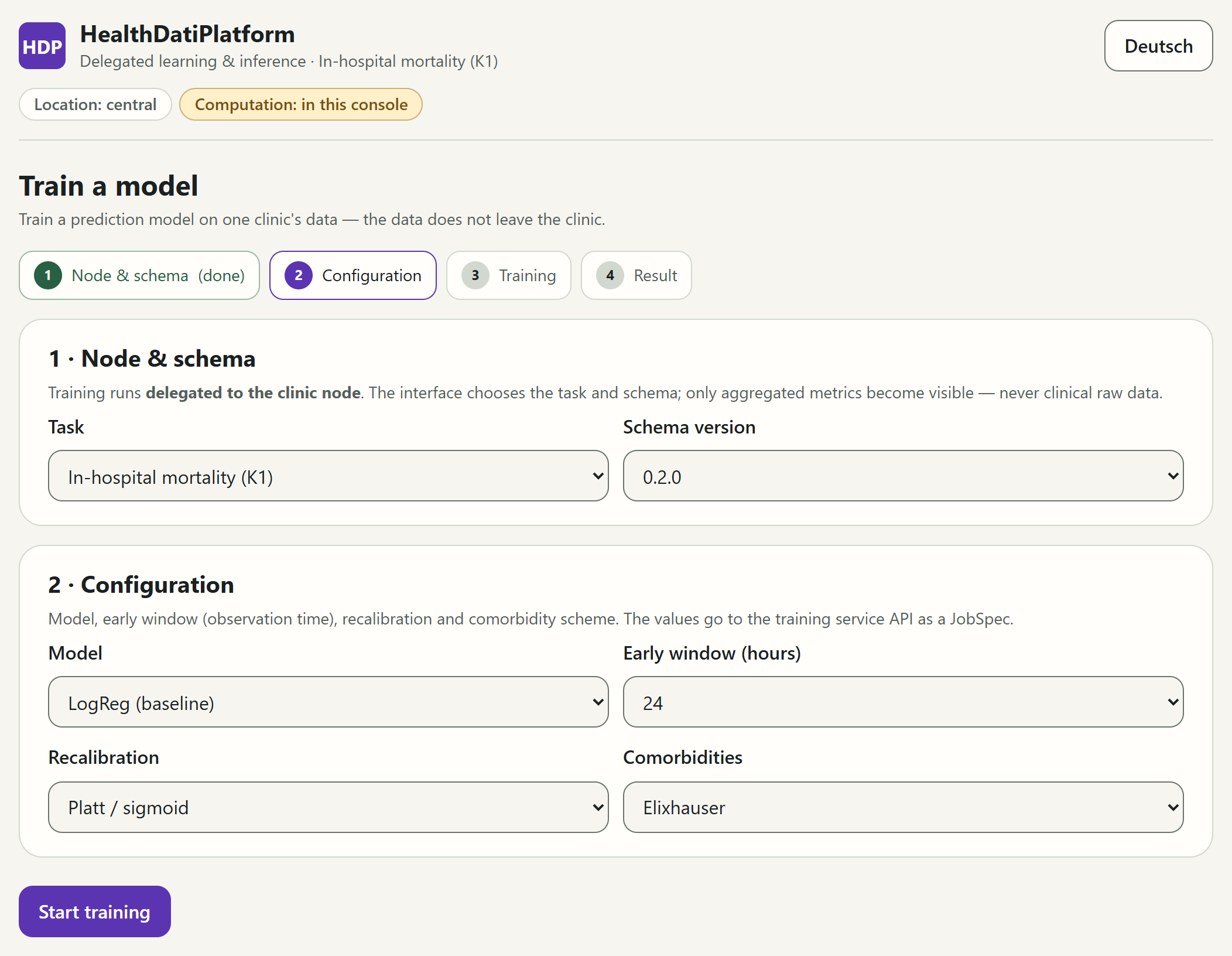
In the Node & schema panel, the Task is fixed: In-hospital mortality (K1). The Schema version determines which version of the shared data model the job expects. The newest is preselected.
In the Configuration panel, you choose:
- Model: the method. ‘LogReg (baseline)’ is a logistic regression, ‘LogReg L1 (sparse)’ a variant that makes do with fewer features, and ‘GBDT’ a method built from many small decision trees.
- Early window (hours): whether the model uses values from the first 24 or the first 48 hours after admission.
- Recalibration: how the model's risk values are adjusted afterwards to match the observed rates. ‘Platt / sigmoid’ is preselected.
- Comorbidities: the scheme that groups pre-existing conditions: Elixhauser, Charlson or both.
The defaults suit a first attempt. Click Start training.
While the training runs
The platform hands the job to a clinic node, which runs the training on site. The interface only sees the status and, at the end, aggregated metrics, never the data themselves.
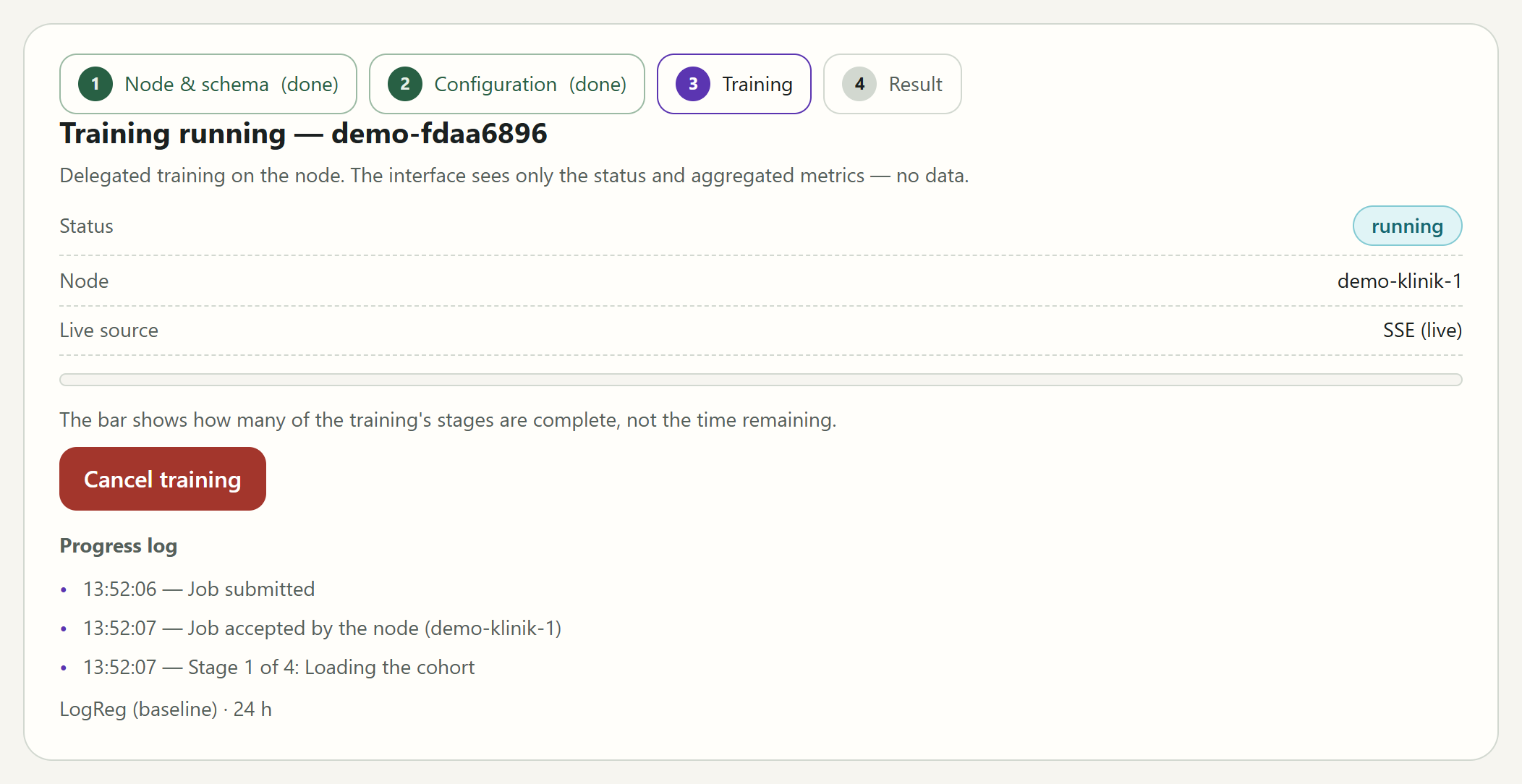
- The status changes from submitted through accepted and running to completed.
- Node names the clinic node that runs the training,
demo-klinik-1in the demo. - The Progress log lists, with the time, what happens at the node: the job is submitted and accepted by the node, then four stages follow, ‘Loading the cohort’, ‘Fitting the model’, ‘Calibrating the model’ and ‘Computing the metrics’.
In the demo, a training run takes about six seconds. Cancel training requests that a running training stop early: the node stops at the next stage boundary, and the current stage still finishes. If the training is done by then, the interface still shows the result on request.
Read the result
When the training has finished, the interface shows the Result.
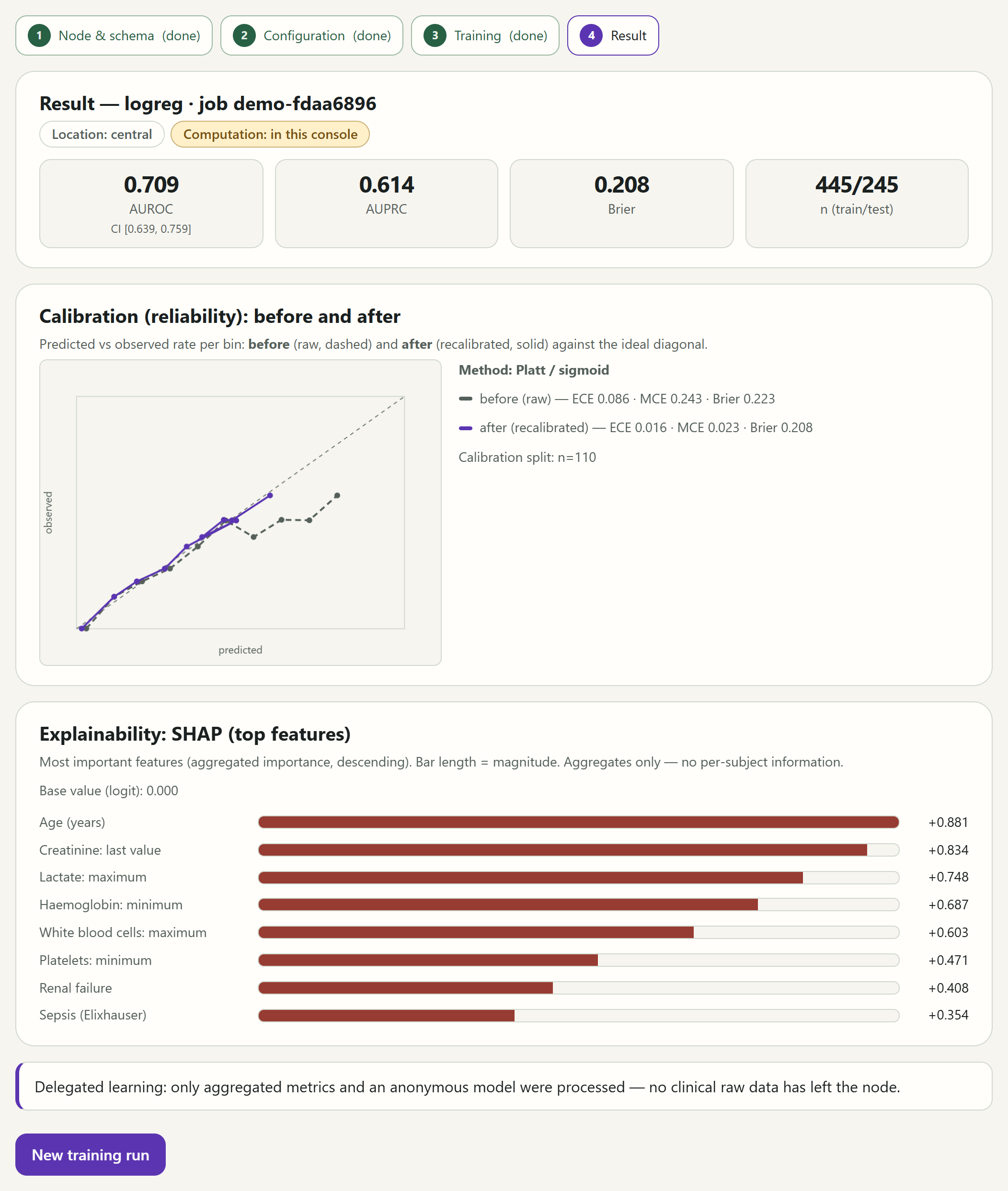
The four metrics at the top describe how well the model performs on test data that were not used for training:
- AUROC: how well the model separates cases with and without the outcome. 0.5 corresponds to chance, 1 to perfect separation. The confidence interval appears below it.
- AUPRC: how well the model finds the rare cases with the outcome without raising too many false alarms. For rare outcomes, it is more informative than AUROC.
- Brier: the mean squared difference between the estimated risk and the actual outcome. The smaller, the better.
- n (train/test): how many cases were used for training and for testing.
Calibration (reliability): before and after shows whether the estimated risks match the observed rates. Where a curve lies on the finely dashed diagonal, they agree. The dashed curve shows the model before recalibration, the solid one after.
Explainability: SHAP (top features) shows which features contributed most to the prediction across all cases, aggregated and without any information about individual people. ‘Creatinine: last value’, for example, is the last creatinine value measured in the early window, and ‘Sepsis (Elixhauser)’ is sepsis as a pre-existing condition according to the Elixhauser scheme.
New training run takes you back to the settings.
Part 2: Assess a risk
Model and warning threshold
Open Assess risk. The interface guides you through three steps: enter values, start the evaluation, read the result.
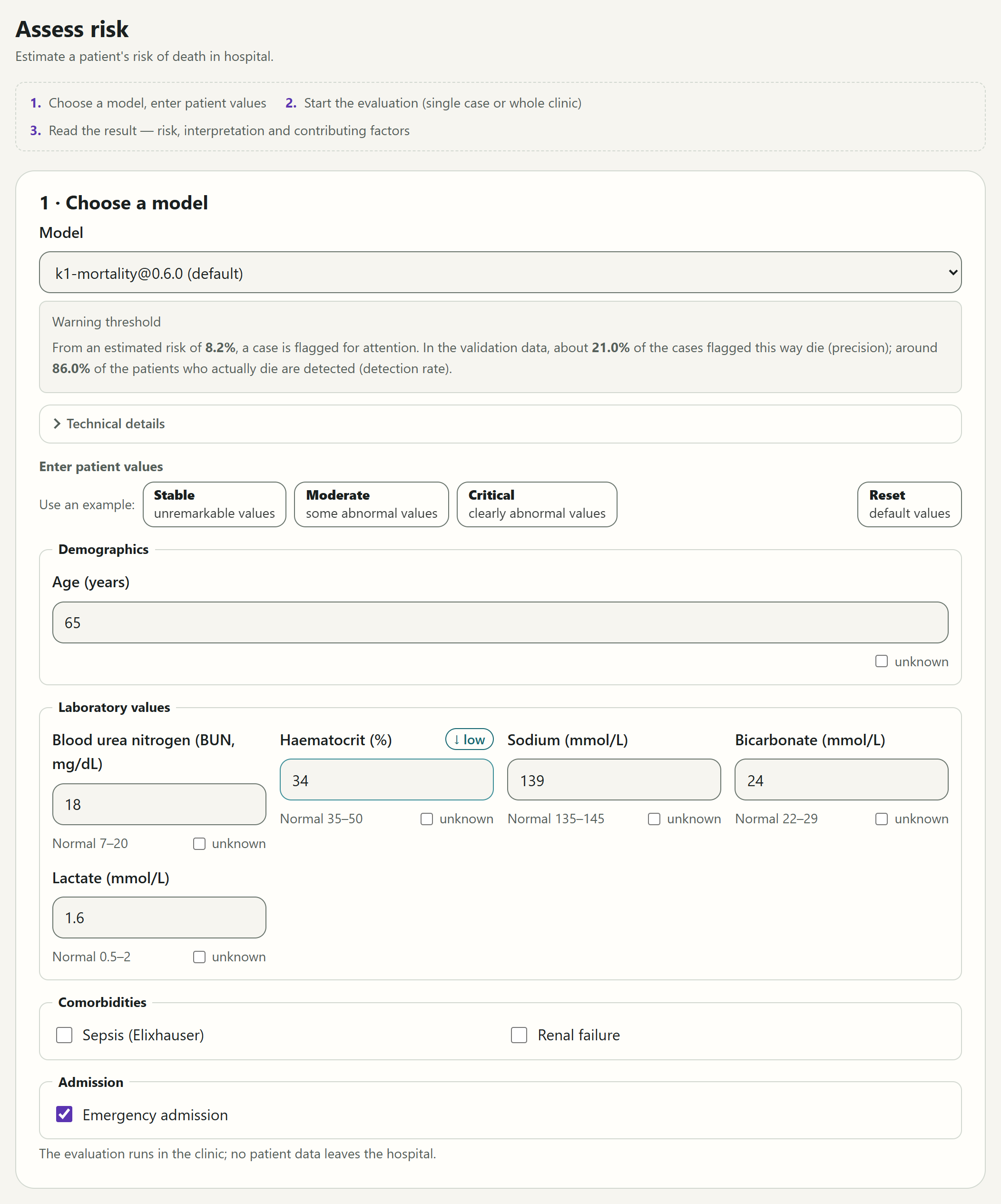
In the Choose a model panel, the standard model is preselected. You do not choose a clinic: Assess risk runs in a clinic and names it at the top as its location.
The Warning threshold box explains when a case is flagged. In the demo, the threshold is ‘8.2%’: from this estimated risk upwards, a case is flagged for attention. Of the cases flagged this way, about 21% died in the evaluation; that is the Precision. Around 86% of those who actually died are detected; that is the Detection rate. Under Technical details, technically minded readers find details about the model.
Enter patient values
Under Enter patient values, there are nine values in four groups: demographics, laboratory values, pre-existing conditions and admission. Below each laboratory value is its reference range. If a value lies outside it, the interface marks it ↓ low or ↑ high.
- If you don't know a numeric value, tick unknown below the field. The platform then calculates with a normal value, and the result points out that the assessment is less certain. For the comorbidities and the admission, an empty box means ‘no’.
- An implausible value, such as an age of 200 years, blocks the calculation until it is corrected or marked as unknown.
Use an example fills all fields with one of three example cases: Stable, Moderate or Critical. Reset restores the defaults and removes a result from the screen.
Calculate a single case
Choose the example case Critical. Above the Start the evaluation panel, Single case is already selected. Click Calculate risk.
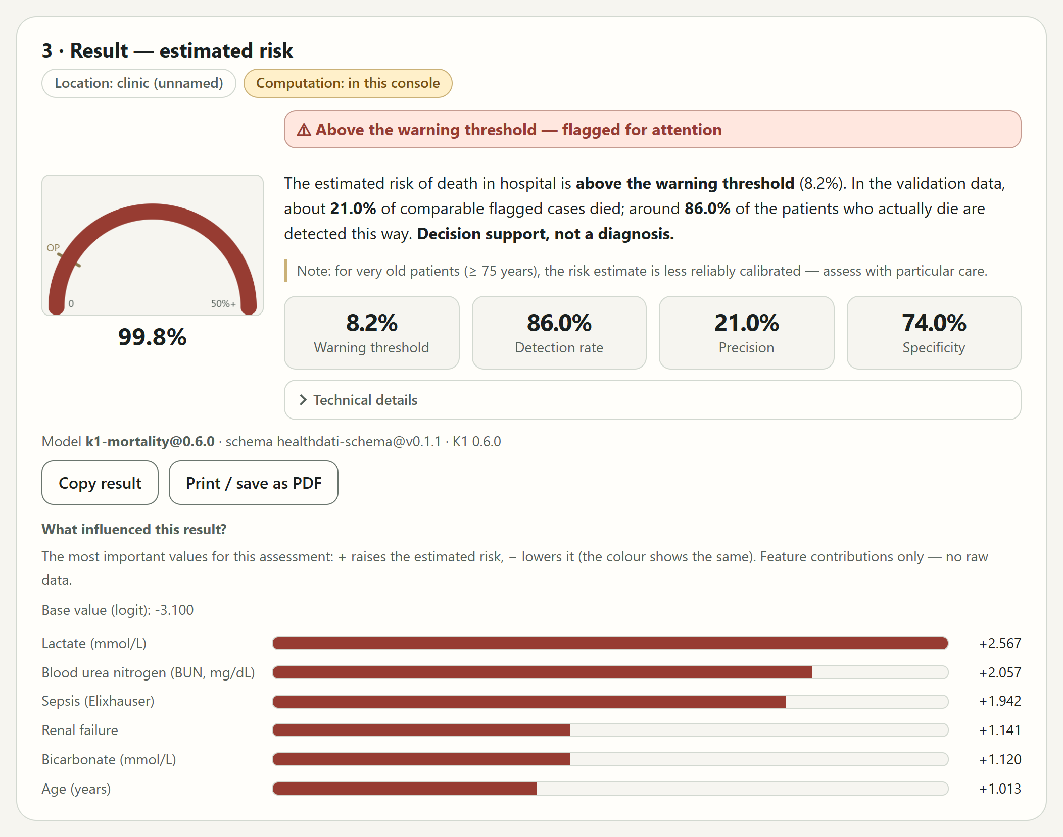
How to read the result:
- The half-circle gauge and the large value below it show the estimated risk, here ‘99.8%’. The scale runs to 50%, and the mark ‘OP’ is the warning threshold.
- Next to it, the interface states whether the case is flagged, here Above the warning threshold — flagged for attention. A short text puts the result into context.
- The cards show the warning threshold's metrics in percent: Warning threshold, Detection rate, Precision and Specificity.
- What influenced this result? shows the most important values for this case. A plus raises the estimated risk, a minus lowers it.
Copy result copies the result as text, for example for a handover. Print / save as PDF creates a printout. Both state the location and the computation. The printout does not contain the patient values entered.
Now click Reset and then Calculate risk again. With the defaults, the risk is ‘2.9%’, which is Below the warning threshold — not flagged.
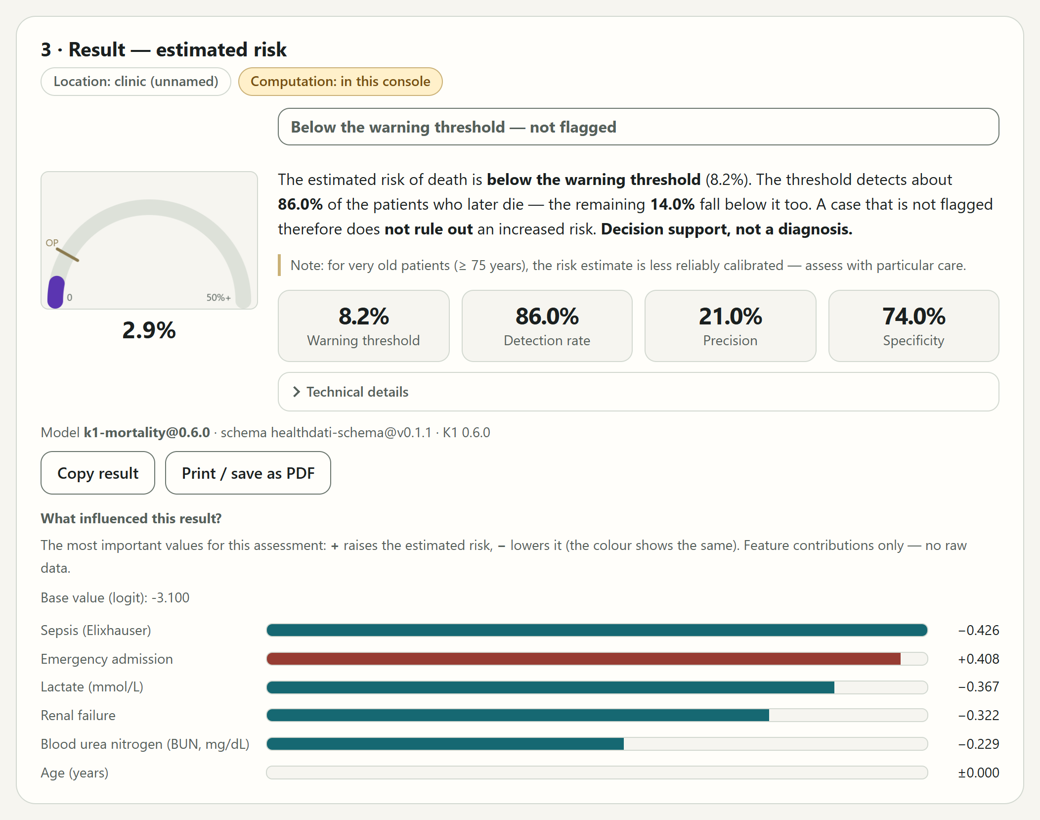
Not flagged does not mean safe. The warning threshold detects about 86% of those who later die; the other 14% also lie below it. That is why the marking is deliberately grey rather than green.
If any values were unknown, the result says how many and that the assessment is correspondingly less certain. Every result also reminds you that the estimate is less reliably calibrated for very old patients, aged 75 and over.
Assess a whole clinic
Above the Start the evaluation panel, switch to Whole clinic. Dataset lists the datasets the clinic node has released for cohorts; the demo has three, ‘Demo A’ to ‘Demo C’. Leave ‘Demo A’ selected and click Start cohort inference. The platform then assesses all cases of this dataset and shows only totals and distributions, never the values of individual patients.
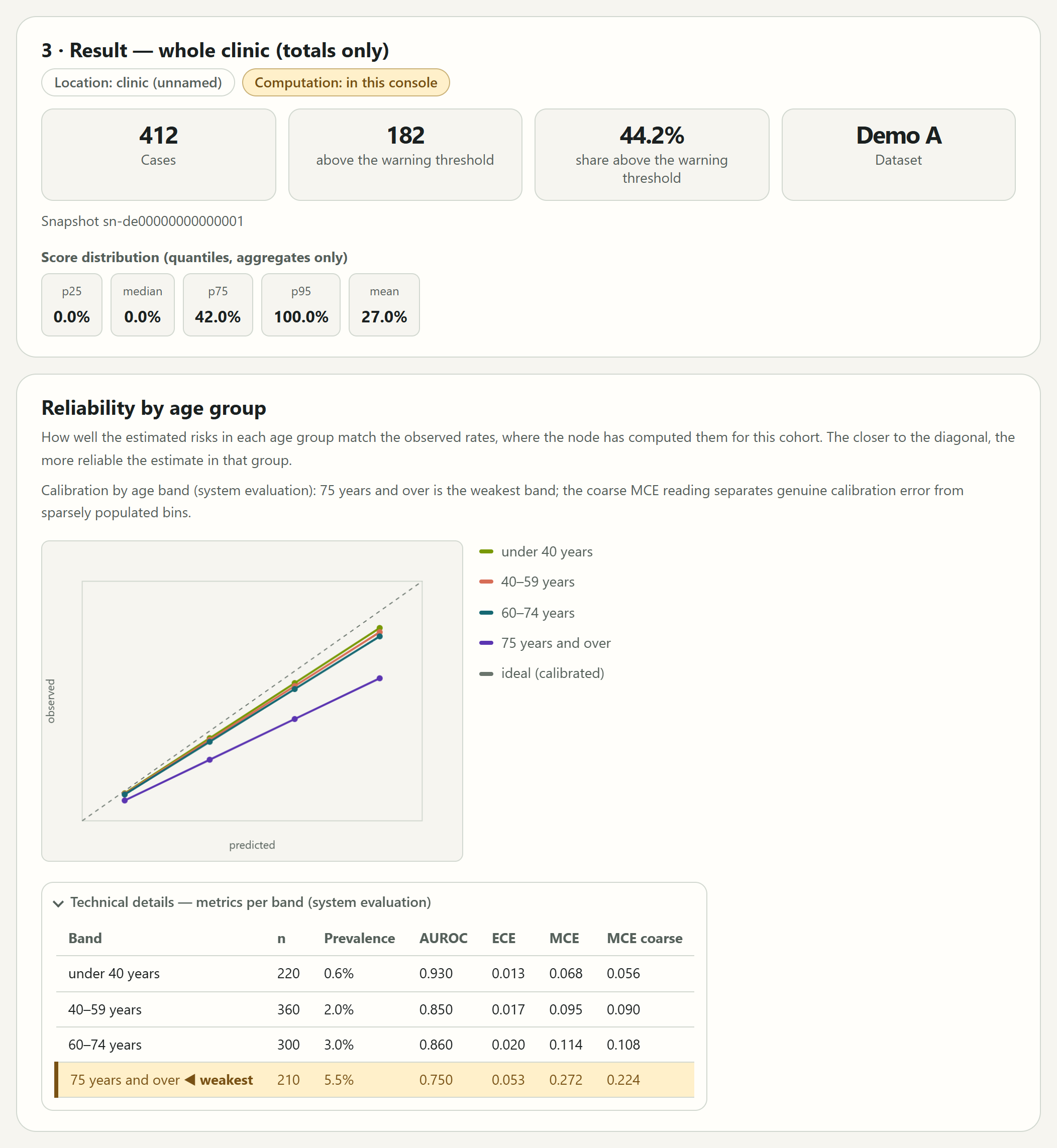
- The cards at the top show the number of cases, how many of them lie above the warning threshold, what share that is, and the dataset.
- The score distribution shows the estimated risks as quantiles, p25, median, p75 and p95, and as their mean, in whole percentage points.
- Reliability by age group shows how well the estimated risks match the observed rates in each age group. The closer to the diagonal, the more reliable. The table under Technical details marks the age group with the weakest calibration as weakest; in the demo, that is the group aged 75 and over.
Putting the result in context
The warning threshold's four metrics describe how the model behaved in the evaluation. In the demo:
| Metric | Meaning | Demo |
|---|---|---|
| Warning threshold | From this estimated risk upwards, a case is flagged. | 8.2% |
| Detection rate | Share of those who actually die who are flagged (sensitivity) | 86.0% |
| Precision | Share of flagged cases who actually die (PPV) | 21.0% |
| Specificity | Share of survivors who are correctly not flagged | 74.0% |
Worth keeping in mind:
- A warning threshold is a trade-off. A lower threshold detects more of those who die, but also flags more cases who survive. According to the technical details, this threshold was set with the cost ratio ‘FN:FP=10:1’: a missed death weighs ten times as much as a false alarm.
- A precision of 21% means that about one in five flagged cases died in the evaluation. The flag directs attention; it does not predict that someone will die.
- A case that is not flagged does not rule out an increased risk.
Running the demo yourself
The demo runs on your own computer. For this you need the platform's source code, which is available to project members, as well as Node.js 24 or later and Python 3.10 or later. In the platform/software/frontend directory, first build the interface and install the Python packages, ideally in a virtual environment:
cd web
npm ci
npm run build
cd ..
pip install -r requirements-demo.txt
Then start the two interfaces as a demo, each in its own terminal. HDP_DEMO=1 selects the demo mode explicitly; without it, and without a connection to the platform, the interfaces do not start:
HDP_DEMO=1 uvicorn app.main:app --port 8080
HDP_DEMO=1 uvicorn inference_app.main:app --port 8081
On Windows, first set $env:HDP_DEMO = "1" in PowerShell and leave out HDP_DEMO=1 before uvicorn.
Train a model is now available at http://127.0.0.1:8080, and Assess risk at http://127.0.0.1:8081. Started this way, both can only be reached from your own computer. How to install the platform at a site, connected to its clinic node, is described on the installation page.
What comes next
At a participating site, both interfaces are connected to the platform and the clinic node; the top then reads Computation: connected services, and Assess risk names the clinic as its location. Training and assessment run inside the hospital, and no patient data leave the clinic. In this version, Assess risk there still shows the demo's model list, input fields and warning threshold, and says so; the score always comes from the node's model. The architecture page shows how the components fit together; the installation page describes how to install the platform at a site.
The user guide, also available as a PDF, explains what every value, message and measure of the two interfaces means.